Linear Regression: A Deep Dive into Assumptions, Interpretation, and Evaluation

Linear regression is a fundamental and widely used statistical and machine learning technique for modeling the relationship between a dependent variable (also called the target or response variable) and one or more independent variables (also called predictors, features, or explanatory variables). It assumes a linear relationship between the variables, meaning that the change in the dependent variable is proportional to the change in the independent variables. This article provides a thorough explanation of linear regression, including its underlying assumptions, how to interpret the model's coefficients, how to evaluate its performance, and practical Python examples.
1. The Linear Regression Model
The basic linear regression model can be expressed as:
Y = β₀ + β₁X₁ + β₂X₂ + ... + βₚXₚ + ε
Where:
- Y: The dependent variable (the variable we are trying to predict).
- X₁, X₂, ..., Xₚ: The independent variables (the predictors).
- β₀: The intercept (the value of Y when all X's are 0).
- β₁, β₂, ..., βₚ: The coefficients (or weights) for each independent variable. These represent the change in Y for a one-unit change in the corresponding X, holding all other X's constant.
- ε: The error term (or residual), which represents the difference between the actual value of Y and the value predicted by the model. This captures all the factors affecting Y that are not included in the model.
Types of Linear Regression
- Simple Linear Regression: One independent variable.
- Multiple Linear Regression: Two or more independent variables.
2. Assumptions of Linear Regression
For linear regression to produce reliable and valid results, several key assumptions must be met (or at least reasonably approximated). Violating these assumptions can lead to biased coefficients, inaccurate predictions, and incorrect inferences.
- 1. Linearity: The relationship between the independent variables and the dependent variable is linear. This means that a one-unit change in an independent variable results in a constant change in the dependent variable, regardless of the values of the other independent variables.
- Checking: Scatter plots of each independent variable against the dependent variable. Look for non-linear patterns (curves, etc.).
- Addressing: Transform variables (e.g., logarithmic, square root, polynomial transformations), or use a non-linear model.
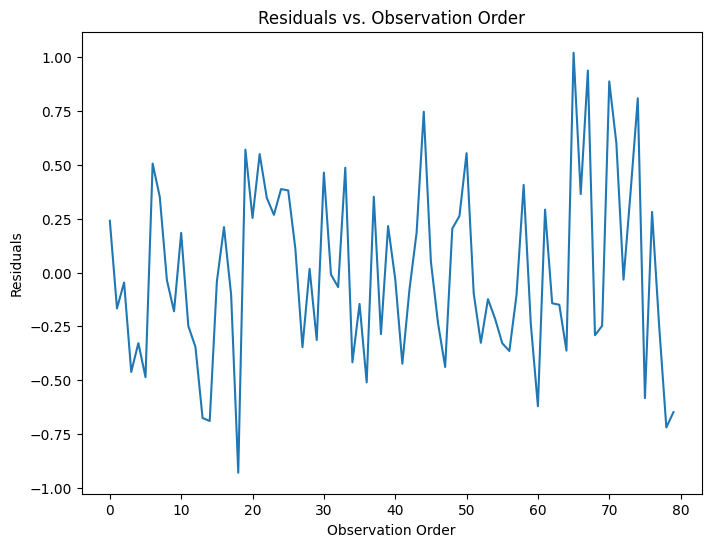
- 2. Independence of Errors: The error terms (residuals) are independent of each other. This means that the error for one observation does not predict the error for another observation. This is particularly important in time-series data.
- Checking: Durbin-Watson test, plot of residuals against time (for time-series data), plot of residuals against predicted values. Look for patterns (autocorrelation).
- Addressing: For time-series data, use time-series models (e.g., ARIMA). For other types of dependence, consider using generalized least squares or mixed-effects models.
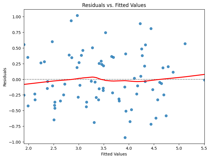
- 3. Homoscedasticity (Constant Variance of Errors): The variance of the error terms is constant across all levels of the independent variables. This means that the spread of the residuals is the same for all predicted values.
- Checking: Plot of residuals against predicted values (or against each independent variable). Look for a "funnel" shape (variance increasing or decreasing with predicted values). Breusch-Pagan test, White test.
- Addressing: Transform the dependent variable (e.g., logarithmic transformation), use weighted least squares.
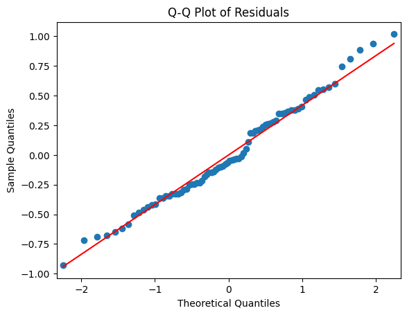
- 4. Normality of Errors: The error terms are normally distributed. This assumption is important for hypothesis testing and confidence interval estimation.
- Checking: Histogram of residuals, Q-Q plot of residuals, Shapiro-Wilk test.
- Addressing: Transform the dependent variable or use robust regression techniques. Note: This assumption is less critical for large sample sizes due to the Central Limit Theorem.
- 5. No Perfect Multicollinearity: The independent variables are not perfectly correlated with each other. High multicollinearity can make it difficult to estimate the individual effects of the independent variables and can lead to unstable coefficient estimates.
- Checking: Correlation matrix of independent variables, Variance Inflation Factor (VIF). VIF values greater than 5 or 10 are often considered problematic.
- Addressing: Remove one or more of the highly correlated variables, combine correlated variables into a single variable, use principal component analysis (PCA), or use ridge regression.
3. Interpreting Coefficients
The coefficients (β₁, β₂, ..., βₚ) in a linear regression model represent the estimated change in the dependent variable (Y) for a one-unit increase in the corresponding independent variable (X), holding all other independent variables constant.
- Intercept (β₀ = 50,000): The estimated price of a house with 0 square footage and 0 bedrooms (this may not be practically meaningful, but it's the baseline).
- SquareFootage Coefficient (β₁ = 100): For every one-square-foot increase in house size, the estimated price increases by $100, holding the number of bedrooms constant.
- Bedrooms Coefficient (β₂ = 20,000): For every additional bedroom, the estimated price increases by $20,000, holding the square footage constant.
- Important Considerations:
- Units: The interpretation of a coefficient depends on the units of the independent and dependent variables.
- Causation: Correlation does not equal causation. Even if a linear regression model shows a strong relationship between two variables, it doesn't necessarily mean that one variable causes the other.
- Statistical Significance: Not all coefficients are statistically significant. We use p-values and confidence intervals to assess whether a coefficient is significantly different from zero.
Example: Suppose we have a model predicting house price (Y) based on square footage (X₁) and number of bedrooms (X₂):
Price = 50,000 + 100 * SquareFootage + 20,000 * Bedrooms
4. Evaluating Linear Regression Models
Several metrics are used to evaluate the performance of a linear regression model:
- R-squared (Coefficient of Determination): Measures the proportion of variance in the dependent variable that is explained by the model. Ranges from 0 to 1. Higher values indicate a better fit.
- Adjusted R-squared: A modified version of R-squared that adjusts for the number of predictors in the model. This is useful for comparing models with different numbers of predictors.
- Mean Squared Error (MSE): The average of the squared differences between the predicted and actual values. Lower values indicate better performance.
- Root Mean Squared Error (RMSE): The square root of the MSE. Has the same units as the dependent variable, making it more interpretable.
- Mean Absolute Error (MAE): The average of the absolute differences between the predicted and actual values. Less sensitive to outliers than MSE/RMSE.
- Residual Plots: Check the assumptions of the linear model.
5. Python Code Example (using Scikit-learn and Statsmodels)
import numpy as np
import pandas as pd
import matplotlib.pyplot as plt
import seaborn as sns
from sklearn.model_selection import train_test_split
from sklearn.linear_model import LinearRegression
from sklearn.metrics import mean_squared_error, r2_score, mean_absolute_error
import statsmodels.api as sm
from statsmodels.stats.outliers_influence import variance_inflation_factor

# --- Generate Sample Data ---
np.random.seed(42)
n_samples = 100
X = np.random.rand(n_samples, 3)  # 3 independent variables
# Create a linear relationship with some noise
y = 2 + 1.5 * X[:, 0] - 0.8 * X[:, 1] + 2.2 * X[:, 2] + np.random.randn(n_samples) * 0.5

# --- Create a Pandas DataFrame (optional, but good for visualization) ---
df = pd.DataFrame(X, columns=['X1', 'X2', 'X3'])
df['y'] = y

# --- Split Data into Training and Testing Sets ---
X_train, X_test, y_train, y_test = train_test_split(X, y, test_size=0.2, random_state=42)

# --- Scikit-learn Linear Regression ---
model_sklearn = LinearRegression()
model_sklearn.fit(X_train, y_train)

# Make predictions
y_pred_sklearn = model_sklearn.predict(X_test)

# Evaluate the model (Scikit-learn)
print("Scikit-learn Model:")
print("  R-squared:", r2_score(y_test, y_pred_sklearn))
print("  MSE:", mean_squared_error(y_test, y_pred_sklearn))
print("  RMSE:", np.sqrt(mean_squared_error(y_test, y_pred_sklearn)))
print("  MAE:", mean_absolute_error(y_test, y_pred_sklearn))
print("  Coefficients:", model_sklearn.coef_)
print("  Intercept:", model_sklearn.intercept_)


# --- Statsmodels Linear Regression (for more detailed statistics) ---
X_train_sm = sm.add_constant(X_train)  # Add a constant (intercept) to the model
model_statsmodels = sm.OLS(y_train, X_train_sm)
results = model_statsmodels.fit()

# Print model summary
print("\nStatsmodels Model Summary:")
print(results.summary())

# --- Check for Multicollinearity (using VIF) ---
vif_data = pd.DataFrame()
vif_data["feature"] = ['const'] + [f'X{i+1}' for i in range(X_train.shape[1])]
vif_data["VIF"] = [variance_inflation_factor(X_train_sm, i) for i in range(X_train_sm.shape[1])]
print("\nVariance Inflation Factors (VIF):")
print(vif_data)

# --- Residual Analysis (using Statsmodels)---

# 1. Linearity and Homoscedasticity: Residuals vs. Fitted Values
plt.figure(figsize=(8, 6))
sns.residplot(x=results.fittedvalues, y=results.resid, lowess=True, line_kws={'color': 'red'})
plt.xlabel("Fitted Values")
plt.ylabel("Residuals")
plt.title("Residuals vs. Fitted Values")
plt.show()

# 2. Normality: Q-Q Plot of Residuals
plt.figure(figsize=(8, 6))
sm.qqplot(results.resid, line='s')  # 's' for standardized line
plt.title("Q-Q Plot of Residuals")
plt.show()

# 3. Independence (if you have a time or sequence component):  Residuals vs. Order
# (Assuming data is already in the correct order)
if True: # Change this to True if there is any ordering
	plt.figure(figsize=(8, 6))
	plt.plot(results.resid)
	plt.xlabel("Observation Order")
	plt.ylabel("Residuals")
	plt.title("Residuals vs. Observation Order")
	plt.show()
Output of the code:
Scikit-learn Model:
  R-squared: 0.5305797499575091
  MSE: 0.5043481201525745
  RMSE: 0.7101747110060836
  MAE: 0.5521899575286403
  Coefficients: [ 1.55294884 -0.837697    2.54302962]
  Intercept: 1.9574947791835386

Statsmodels Model Summary:
                            OLS Regression Results
==============================================================================
Dep. Variable:                      y   R-squared:                       0.810
Model:                            OLS   Adj. R-squared:                  0.802
Method:                 Least Squares   F-statistic:                     107.7
Date:                Wed, 12 Feb 2025   Prob (F-statistic):           2.72e-27
Time:                        08:03:25   Log-Likelihood:                -43.811
No. Observations:                  80   AIC:                             95.62
Df Residuals:                      76   BIC:                             105.2
Df Model:                           3
Covariance Type:            nonrobust
==============================================================================
                 coef    std err          t      P>|t|      [0.025      0.975]
------------------------------------------------------------------------------
const          1.9575      0.151     12.979      0.000       1.657       2.258
x1             1.5529      0.171      9.106      0.000       1.213       1.893
x2            -0.8377      0.155     -5.421      0.000      -1.145      -0.530
x3             2.5430      0.167     15.194      0.000       2.210       2.876
==============================================================================
Omnibus:                        1.625   Durbin-Watson:                   1.692
Prob(Omnibus):                  0.444   Jarque-Bera (JB):                1.627
Skew:                           0.276   Prob(JB):                        0.443
Kurtosis:                       2.571   Cond. No.                         6.23
==============================================================================

Notes:
[1] Standard Errors assume that the covariance matrix of the errors is correctly specified.

Variance Inflation Factors (VIF):
  feature       VIF
0   const  9.875050
1      X1  1.013455
2      X2  1.004332
3      X3  1.015770


Key Code Explanations:
- Imports: Imports necessary libraries (NumPy for numerical operations, Pandas for data manipulation, Matplotlib and Seaborn for plotting, Scikit-learn for machine learning, Statsmodels for statistical modeling).
- Data Generation: Creates a synthetic dataset with a linear relationship and added noise. In a real application, you would load your data.
- Train/Test Split: Splits the data into training and testing sets using
train_test_split. - Scikit-learn Model:
LinearRegression(): Creates a linear regression model object.fit(): Trains the model on the training data.predict(): Makes predictions on the test data.- Evaluation metrics (R-squared, MSE, RMSE, MAE) are calculated using functions from
sklearn.metrics.
- Statsmodels Model:
sm.add_constant(): Adds a column of 1s to the feature matrix to represent the intercept term.sm.OLS(): Creates an Ordinary Least Squares (OLS) linear regression model.fit(): Fits the model to the data.results.summary(): Provides a comprehensive summary of the model, including coefficients, standard errors, p-values, confidence intervals, R-squared, and other statistics.
- Multicollinearity check
- Calculates the Variance Inflation Factor for each independent variable.
- Residual Analysis
- Create residual plots to check the assumptions of the linear regression model.
6. Conclusion
Linear regression is a powerful and versatile tool for modeling linear relationships between variables. However, it's essential to understand its assumptions, interpret the coefficients correctly, and evaluate the model's performance using appropriate metrics. By following the steps outlined in this article and utilizing the provided Python code examples, you can effectively apply linear regression to your own data analysis and machine learning tasks. Remember to always check the assumptions and critically evaluate your results.
References
[1] James, G., Witten, D., Hastie, T., & Tibshirani, R. (2013). An Introduction to Statistical Learning: with Applications in R. Springer.
[2] Hastie, T., Tibshirani, R., & Friedman, J. (2009). The Elements of Statistical Learning: Data Mining, Inference, and Prediction (2nd ed.). Springer.
[3] Montgomery, D. C., Peck, E. A., & Vining, G. G. (2012). Introduction to linear regression analysis (5th ed.). John Wiley & Sons.
[4] Draper, N. R., & Smith, H. (1998). Applied regression analysis (3rd ed.). John Wiley & Sons.
[5] Kutner, M.H., Nachtsheim, C.J., Neter, J., Li, W. (2005) Applied Linear Statistical Models (5th ed.). McGraw-Hill/Irwin
Additional reads:


Comments ()