Decision Trees for Classification and Regression: A Comprehensive Guide

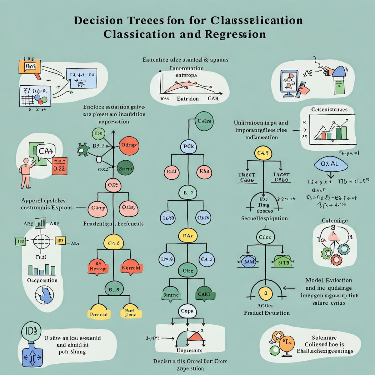
Decision trees are a popular machine learning algorithm known for their simplicity and interpretability. They are used for both classification and regression tasks, making them a versatile tool for various applications. This article delves into the inner workings of decision trees, exploring how they split data, make predictions, and the different variants of this powerful algorithm.

A decision tree is a flowchart-like structure that represents a series of decisions (or tests) based on the features of a dataset. Each internal node in the tree represents a test on an attribute (feature), each branch represents the outcome of the test, and each leaf node (terminal node) represents a class label (in classification) or a predicted value (in regression).

Analogy: Imagine you're trying to decide whether to play tennis outside. You might consider factors like:

• Outlook: Sunny, Overcast, or Rainy?
• Temperature: Hot, Mild, or Cool?
• Humidity: High or Normal?
• Windy: True or False?

A decision tree would represent this decision-making process as a series of nested "if-then-else" rules, leading to a final decision (Play Tennis or Don't Play Tennis).

How Decision Trees is Built

A decision tree is a tree-like structure where:

• Nodes: Represent decisions or tests on features (attributes) of the data.
• Internal Nodes: Represent a test on an attribute.
• Branches: Represent the outcome of a test (e.g., "Yes" or "No", or a range of values).
• Leaf Nodes (Terminal Nodes): Represent the final prediction (a class label in classification or a numerical value in regression).
• Root Node: Represents the entire dataset.

The process of building a decision tree involves recursively partitioning the data based on feature values to create increasingly homogeneous subsets. This is done through a process known as recursive partitioning.

Recursive Partitioning

1. Start at the Root: The entire dataset is considered at the root node.
2. Find the Best Split: The algorithm searches for the "best" feature and the "best" split point on that feature to divide the data. "Best" is determined by an impurity measure (explained below).
3. Split the Data: The data is split into subsets (child nodes) based on the chosen split.
4. Recurse: Steps 2 and 3 are repeated for each child node until a stopping criterion is met (e.g., maximum tree depth, minimum samples per leaf, or impurity below a threshold).

How Decision Trees Split Data

Decision trees partition data into smaller and more homogeneous subsets based on the values of different features. This process, known as recursive binary splitting, starts with the root node, which represents the entire dataset. The algorithm then selects the feature that best separates the data based on a specific criterion, such as information gain or Gini impurity. Decision trees aim to create "pure" nodes, where the majority of instances belong to the same class. The splitting process continues until most nodes are pure or a stopping criterion is met.  

Splitting Criteria

Gini Impurity: Measures the probability of misclassifying a randomly chosen element from the dataset if it were randomly labeled according to the class distribution in the subset. A lower Gini impurity indicates a purer node. For example, imagine a basket of apples and oranges. If the basket contains only apples, the Gini impurity is 0, as there's no chance of misclassifying a fruit. As we add oranges to the basket, the Gini impurity increases, reflecting the higher probability of misclassification.  

Equation:
\[ Gini(t) = 1 - \Sigma(p(i|t))^2 \]

Where, \(t\) is a node. \(p(i|t)\) is the proportion of instances belonging to class i at node t. Ranges from 0 (perfect purity) to 0.5 (maximum impurity for a binary classification problem).

Entropy: Quantifies the disorder or uncertainty in a dataset. A lower entropy value represents a more homogeneous subset. Information gain, calculated based on entropy, measures the reduction in entropy achieved by splitting the data based on a particular feature. The higher the information gain, the better the split. Think of a room with toys scattered everywhere. This room has high entropy. As we organize the toys into their respective boxes, the entropy decreases, reflecting the increased order.

Equation:
\[Entropy(t) = - Σ [p(i|t) * log₂(p(i|t))]\]

Where, \(t\) is a node. \(p(i|t)\) is the proportion of instances belonging to class \(i\) at node \(t\). Ranges from 0 (perfect purity) to 1 (maximum impurity for a binary classification problem). Measures the "disorder" or "randomness" in the data.

Information Gain: The difference between the entropy of the parent node and the weighted average entropy of the child nodes after a split. The algorithm chooses the split that maximizes information gain.  

Equation:
\[Information Gain = Entropy(parent) - Σ [(Nᵢ / N) * Entropy(childᵢ)]\]

Where \(N_i\) is the number of samples in the ith child and \(N\) is the number of samples in the parent.

Variance Reduction: For regression tasks, variance reduction is used as the splitting criterion. The algorithm selects the split that minimizes the variance of the target variable within each child node.  

Handling Different Data Types

Decision trees can handle both numerical and categorical data.  

• Numerical Data: For numerical features, the algorithm identifies thresholds or cut-off points that best split the data. For instance, if the feature is "age," the split could be "age < 25" and "age >= 25." 
• Categorical Data: Categorical features are split based on different groupings of categories. The algorithm evaluates different combinations of categories to find the split that maximizes the chosen splitting criterion.  

Data Fragmentation

As the decision tree grows deeper, it can lead to data fragmentation, where the number of instances in each node becomes very small. This can result in overfitting, where the tree becomes too specific to the training data and fails to generalize well to new, unseen data.  

To illustrate this, imagine a decision tree for classifying animals. If the tree keeps splitting based on very specific features like "has stripes" or "has a long tail," it might end up with leaf nodes containing only one or two animals. This highly specific tree might accurately classify the animals in the training data but fail to classify new animals that don't exactly match those specific features.

How Decision Trees Make Predictions

Once the decision tree is constructed, making predictions is a straightforward process. For a given input, the algorithm traverses the tree from the root node down to a leaf node based on the values of the input features. Each internal node represents a decision based on a specific feature, and the branches represent the possible outcomes of that decision. The leaf node reached at the end of this traversal contains the final prediction.  

Traversal Process

The algorithm starts at the root node and evaluates the feature specified at that node. Based on the value of the input feature, it follows the corresponding branch to the next node. This process continues until a leaf node is reached.

Prediction at Leaf Node

The leaf node contains the final prediction, which is typically the most common class label (for classification) or the average value (for regression) of the training instances that ended up in that node.

For instance, consider a decision tree for predicting whether a customer will purchase a product. The tree might start with a question like "Is the customer's age greater than 30?" If the answer is yes, the algorithm follows the corresponding branch. The next node might ask, "Is the customer's income greater than $50,000?" Based on the answer, the algorithm continues down the tree until it reaches a leaf node, which will contain the prediction – either "yes" (will purchase) or "no" (will not purchase).  

Different Variants of Decision Trees

Several variants of decision tree algorithms exist, each with its own approach to constructing and optimizing the tree. Some of the notable ones include:

• ID3 (Iterative Dichotomiser 3): A classic algorithm that uses entropy and information gain to select the best features for splitting. It works well with categorical features but has limitations in handling continuous attributes and is prone to overfitting.  
• C4.5: An improvement over ID3 that uses gain ratio, a modified version of information gain, to reduce bias towards features with many values. It also handles continuous attributes more effectively by creating thresholds for splitting. However, it can still be prone to overfitting, especially with noisy datasets.  
• CART (Classification and Regression Trees): A versatile algorithm used for both classification and regression tasks. It typically uses Gini impurity for classification and variance reduction for regression. CART is known for its ability to handle both numerical and categorical data and is widely used in various applications.  
• CHAID (Chi-square Automatic Interaction Detection): Employs chi-square tests to determine the best splits, making it suitable for analyzing categorical data. It can handle multi-level splits, allowing for more complex relationships to be captured.  
• Oblique Decision Trees: Unlike traditional decision trees that create axis-parallel splits (e.g., "age < 25"), oblique decision trees can create splits at any angle, allowing for more complex decision boundaries. This can improve accuracy but may also increase complexity and reduce interpretability.  

The choice of which decision tree variant to use depends on the specific characteristics of the data and the desired balance between accuracy and interpretability. For instance, when dealing with datasets with many categorical features, CHAID might be a suitable choice. If interpretability is paramount, ID3 or CART might be preferred.

Examples of Decision Trees in Real-World Problems

Decision trees find applications in a wide range of domains, including:

• Healthcare:
  • Diagnosing Diseases: Decision trees can be used to diagnose diseases based on patient symptoms and medical history. For example, a decision tree could be used to predict the likelihood of a patient having a heart attack based on factors like age, cholesterol levels, and family history.  
  • Predicting Patient Outcomes: Decision trees can help predict patient outcomes after surgery or treatment. For instance, a decision tree could predict the likelihood of a patient recovering successfully from a specific type of cancer based on factors like tumor size, stage, and treatment received.  
• Finance:
  • Credit Scoring: Banks and financial institutions use decision trees to assess the creditworthiness of loan applicants. The decision tree analyzes factors like credit history, income, and debt-to-income ratio to predict the likelihood of a borrower defaulting on a loan.  
  • Fraud Detection: Decision trees can be used to detect fraudulent transactions by identifying patterns in data that deviate from normal behavior. For example, a decision tree could be used to flag potentially fraudulent credit card transactions based on factors like transaction amount, location, and purchase history.  
• Marketing:
  • Customer Segmentation: Decision trees can segment customers into different groups based on their demographics, purchase history, and preferences. This allows marketers to tailor their campaigns to specific customer segments, increasing the effectiveness of their marketing efforts.  
  • Targeted Advertising: Decision trees can be used to predict which customers are most likely to respond to a particular advertisement. This allows advertisers to target their ads more effectively, reducing wasted ad spend and improving conversion rates.  
• Retail:
  • Inventory Management: Decision trees can help retailers optimize their inventory levels by predicting demand for different products. This helps prevent stockouts and reduces inventory holding costs.  
  • Sales Forecasting: Decision trees can be used to forecast future sales based on historical data and current market trends. This helps retailers plan their inventory and staffing needs more effectively.  

Advantages of Decision Trees

Decision trees offer several advantages that contribute to their popularity:

• Interpretability: Decision trees are easy to understand and visualize, making them transparent and explainable. This is crucial in applications where understanding the reasoning behind predictions is important, such as medical diagnosis or loan approvals. Simpler decision trees are often preferred for their interpretability, even if they might sacrifice some accuracy compared to more complex models.  
• Handling Non-linearity: They can capture non-linear relationships between features and the target variable, making them suitable for complex datasets where linear models might not perform well.  
• Versatility: They can be used for both classification and regression tasks, handling both numerical and categorical data without the need for extensive data transformations.  
• Minimal Data Preparation: Decision trees often require less data preprocessing compared to other algorithms. They are robust to outliers and can handle missing values effectively, making them suitable for datasets with incomplete or noisy data.  

Pruning Decision Trees

Pruning is a technique used to reduce the size of decision trees by removing sections that provide little to no predictive power. This helps prevent overfitting, where the tree becomes too complex and memorizes the training data instead of learning generalizable patterns.  

There are two main types of pruning:

• Pre-pruning: Involves stopping the growth of the tree early by setting constraints on its depth, the number of samples in a node, or the minimum information gain required for a split. This prevents the tree from becoming too complex and reduces the risk of overfitting. However, it can also lead to underfitting if the stopping criteria are too strict.  
• Post-pruning: Allows the tree to grow to its full depth and then removes branches that do not significantly contribute to the model's accuracy. This approach can be more effective in finding the optimal tree size but can also be more computationally expensive. Common post-pruning techniques include cost-complexity pruning and reduced error pruning.  

Ensemble Methods Utilizing Decision Trees

Ensemble methods combine multiple decision trees to create a more robust and accurate model. Some popular ensemble methods that utilize decision trees include:

• Random Forest: Builds multiple decision trees on different subsets of the data and combines their predictions through majority voting (for classification) or averaging (for regression). This reduces variance and improves the generalization ability of the model.  
• Gradient Boosting Machines: Constructs trees sequentially, where each new tree corrects the errors of the previous ones. This focuses on the instances that were misclassified by previous trees, leading to a more accurate model.  

These ensemble methods often outperform single decision trees by reducing variance and improving generalization.  

Python Code Examples (scikit-learn)

import numpy as np
from sklearn.tree import DecisionTreeClassifier, DecisionTreeRegressor, plot_tree
from sklearn.model_selection import train_test_split
from sklearn.metrics import accuracy_score, mean_squared_error, r2_score
from sklearn.datasets import make_classification, make_regression
import matplotlib.pyplot as plt

# --- Classification Example ---
# Generate synthetic classification data
X_class, y_class = make_classification(n_samples=100, n_features=2, n_informative=2, n_redundant=0, random_state=42)
X_class_train, X_class_test, y_class_train, y_class_test = train_test_split(X_class, y_class, test_size=0.2, random_state=42)

# Create and train a DecisionTreeClassifier
clf = DecisionTreeClassifier(criterion='gini', max_depth=3, random_state=42)  # 'gini' or 'entropy'
clf.fit(X_class_train, y_class_train)

# Make predictions and evaluate
y_class_pred = clf.predict(X_class_test)
accuracy = accuracy_score(y_class_test, y_class_pred)
print(f"Classification Accuracy: {accuracy}")

# Visualize the tree
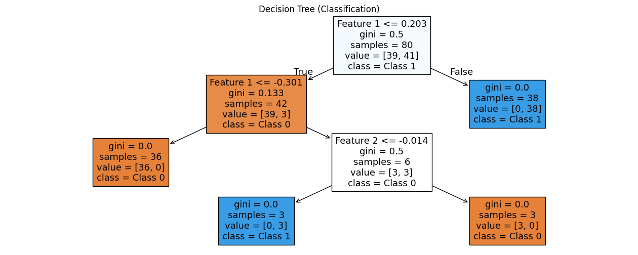
plt.figure(figsize=(12, 8))
plot_tree(clf, filled=True, feature_names=['Feature 1', 'Feature 2'], class_names=['Class 0', 'Class 1'])
plt.title("Decision Tree (Classification)")
plt.show()

# --- Regression Example ---
# Generate synthetic regression data
X_reg, y_reg = make_regression(n_samples=100, n_features=1, noise=0.2, random_state=42)
X_reg_train, X_reg_test, y_reg_train, y_reg_test = train_test_split(X_reg, y_reg, test_size=0.2, random_state=42)

# Create and train a DecisionTreeRegressor
reg = DecisionTreeRegressor(max_depth=3, random_state=42)
reg.fit(X_reg_train, y_reg_train)

# Make predictions and evaluate
y_reg_pred = reg.predict(X_reg_test)
mse = mean_squared_error(y_reg_test, y_reg_pred)
r2 = r2_score(y_reg_test, y_reg_pred)
print(f"Regression MSE: {mse}")
print(f"Regression R^2: {r2}")

# Visualize the tree
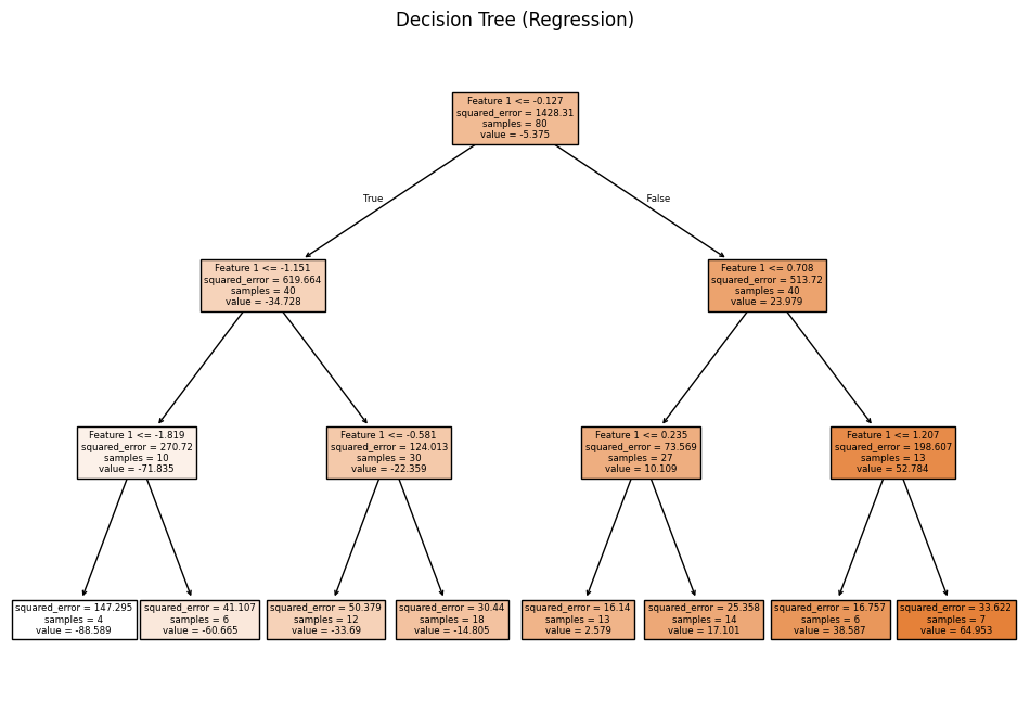
plt.figure(figsize=(12, 8))
plot_tree(reg, filled=True, feature_names=['Feature 1'])
plt.title("Decision Tree (Regression)")
plt.show()

# --- Feature Importance ---
print(f"Classification Feature Importances: {clf.feature_importances_}")
print(f"Regression Feature Importances: {reg.feature_importances_}")

Output:

Classification Accuracy: 0.95

Regression MSE: 41.10652899657141
Regression R^2: 0.9705571251617732

Classification Feature Importances: [0.9249531 0.0750469]
Regression Feature Importances: [1.]

Explanation:

• DecisionTreeClassifier and DecisionTreeRegressor: These are the scikit-learn classes for classification and regression trees, respectively.
• criterion: Specifies the impurity measure ('gini' or 'entropy' for classification). The default for regression is 'squared_error' (which minimizes variance).
• max_depth: Controls the maximum depth of the tree (a key hyperparameter to prevent overfitting).
• random_state: Ensures reproducibility.
• fit: Trains the model.
• predict: Makes predictions.
• accuracy_score, mean_squared_error, r2_score: Evaluation metrics.
• plot_tree: Visualizes the decision tree structure (very helpful for understanding).
• feature_importances_: Provides a measure of the importance of each feature in the tree. Higher values indicate more important features.

Conclusion

Decision trees are a valuable tool in the machine learning arsenal. Their simplicity, interpretability, and versatility make them suitable for a wide range of applications. By understanding how they split data, make predictions, and the different variants and techniques associated with them, data scientists can leverage the power of decision trees to gain insights and build effective predictive models. As the field of artificial intelligence and big data analytics continues to evolve, decision trees are likely to play an even more significant role in extracting knowledge and making informed decisions from complex datasets.

References

• Scikit-learn Documentation: Decision Trees:https://scikit-learn.org/stable/modules/tree.html
• An Introduction to Statistical Learning (ISLR): Chapter 8 covers decision trees. (https://www.statlearning.com/)
• Elements of Statistical Learning (ESL): Chapter 9 provides a more advanced treatment. (https://hastie.su.domains/ElemStatLearn/)
• Breiman, L., Friedman, J. H., Olshen, R. A., & Stone, C. J. (1984). Classification and regression trees. Wadsworth & Brooks/Cole Advanced Books & Software. - The original CART (Classification and Regression Trees) book.  
• Quinlan, J. R. (1986). Induction of decision trees. Machine learning, 1(1), 81-106. - A seminal paper on decision trees (ID3 algorithm).
• Quinlan, J. R. (1993). C4. 5: programs for machine learning. Morgan Kaufmann Publishers Inc.. - Describes the C4.5 algorithm, an improvement over ID3.